WhichLee - An Attack on Numerical Stability in Machine Learning (CTFSGCTF 2021)
Introduction
For CTFSGCTF 2021, I created a problem that was inspired by my current research work at the time. The paper is unfortunately stuck in a limbo and hasn’t met any luck in being published after getting borderline rejected several times, but I thought I should finally write up the actual solution to this problem to clear my head before my next submission. Without further ado, here’s the challenge and the much procrastinated writeup from the challenge author (aka myself).
Challenge Description
Challenge Title: WhichLee
Which Lee do you want to be? Can you be the best Lee of them all?
Find out which Lee you are at this website!
p.s. we are using pytorch 1.8.0+cpu
Hint: Numerical InstabiLEEty
Author: waituck
Solves: 3
The challenge came with a zip file distrib.zip, which contained a pre-trained model leenet.ph and eval.py; the latter is reproduced here below:
#!/usr/bin/env python3

import torch
import torch.nn as nn
from torch.autograd import Function, Variable
from torch.nn.parameter import Parameter
from torchvision import datasets, transforms
import torch.nn.functional as F

import sys

path = sys.argv[1]

NFEATURES=16*16
NHIDDEN=8*8
NCL=5
EPS = 0.00001

# not LeNet
class LeeNet(nn.Module):
    def __init__(self, nFeatures=NFEATURES, nHidden=NHIDDEN, nCl=NCL):
        super().__init__()
        self.fc1 = nn.Linear(nFeatures, nHidden)
        self.fc2 = nn.Linear(nHidden, nCl)

    def forward(self, x):
        nBatch = x.size(0)

        # Normal FC network.
        x = x.view(nBatch, -1)
        x = F.relu(self.fc1(x))
        x = F.relu(self.fc2(x))
        x = F.layer_norm(x, x.size()[1:], eps=1e-50)

        probs = F.softmax(x)

        return probs

# load the model
model = LeeNet()
model.load_state_dict(torch.load("./leenet.ph"))

transform = transforms.Compose([transforms.Resize(16),
                                transforms.CenterCrop(16),
                                transforms.Grayscale(),
                                transforms.ToTensor()])


dataset = datasets.ImageFolder(path, transform=transform)
dataloader = torch.utils.data.DataLoader(dataset, batch_size=1, shuffle=True)
images, labels = next(iter(dataloader))
image = images[0].reshape((1, NFEATURES))

y_pred = model(image)
# no flag for you :P
y_pred[:,0] = torch.min(y_pred) - EPS
decision = torch.argmax(y_pred)
print(str(int(decision)))
Author’s comment: we hope you appreciate the LeNet/LeeNet pun
Users interacted with this python script through the website linked in the description (no longer available, sorry folks). I’ll leave a photo of the website here for those who are curious how it looks like (stolen from duckness).

The website essentially maps the output of the decision to an image of one of our favourite Lees. The code is reproduced below so you have a sense of which lees are available and where the flag is. There’s nothing interesting here other than that, so feel free to skip this snippet.
<html>
    <head>
        <script
            src="https://code.jquery.com/jquery-3.6.0.min.js"
            integrity="sha256-/xUj+3OJU5yExlq6GSYGSHk7tPXikynS7ogEvDej/m4="
            crossorigin="anonymous"></script>

        <script>
            $(function(){
                $('#uploadbtn').on('click', function(){
                    event.preventDefault();
                    $.ajax({
                        url: '/check_lee',
                        type: 'POST',
                        data: $('input[type=file]')[0].files[0],
                        success: function(data){
                            $("#lee").attr("src", `lee${data.class}.png`);
                            if (data.class === 0 && data.flag) {
                                $("#thislee").text(data.flag)
                            } else if (data.class === 1) {
                                $("#thislee").text("You are Bruce LEE! WATAHHHHHHHHHH")
                            } else if (data.class === 2) {
                                $("#thislee").text("You are Bobby LEE! You are super funny")
                            } else if (data.class === 3) {
                                $("#thislee").text("You are LEE Min Ho! You are handsome!")
                            } else if (data.class === 4) {
                                $("#thislee").text("You are Mark LEE! Say no to gambling!")
                            }
                        },
                        error: function() {
                            $("#thislee").text("Request failed! Check the network logs for details.")
                        },
                        cache: false,
                        contentType: false,
                        processData: false
                    });
                });
            });
        </script>
    </head>

    <body>
        <img id="lee" src=""></img>
        <h1 id="thislee"></h1>
        <br />
        <p>Which Lee Are You? (1MB limit, sorry kids)</p>
        <br />
        <form id="fileupload"  method="post" enctype="multipart/form-data">
            <input type="file" name="pic">
        </form>
        <input id="uploadbtn" type="button" value="Upload PNG" name="submit">
    </body>

</html>
The goal is to submit an adversarial image to force the server than runs eval.py to output a class label of 0 corresponding to the flag.
Of course, one of the things you can do at the start is to see if you can cheese the challenge by uploading random images ala Emmel in StacktheFlags2020 (warning NSFW), but you’ll soon come to realize that such attempts are futile for this challenge. This means we actually have to solve the challenge correctly, and we deep dive into the challenge below.
What’s In a Zero Class Label
Anyone with a keen eye will realize this snippet of code in eval.py is the key to getting the flag.
EPS = 0.00001
...
y_pred = model(image)
# no flag for you :P
y_pred[:,0] = torch.min(y_pred) - EPS
decision = torch.argmax(y_pred)
print(str(int(decision)))
It seems to be blocking the flag by manipulating the value of y_pred in the zeroth component. Obviously, this means the value of the zeroth component is extremely important, so let’s try to deep dive into this block of code.
We first note that the output of the model is essentially the output of a softmax function, which maps each component to \((0,1)\), and all component sums to 1. Intuitively, we can interpret this as a probability distribution, but practically, this affects what we can output with a given image. With these constraints in mind, let’s look at what ideas we can play with for y_pred to achieve our target objective.
Idea 1: A Uniform Output
A simple idea is to see what kind of “special” values of y_pred would give us a potentially useful result. One natural train of thought is to force it to output the uniform distribution (i.e. 0.2 on each component of y_pred), and if we argmax over that we could be lucky enough that torch implemented in a way that returns the first entry. Indeed, this is what happens when we quickly check in the Python interpreter:
>>> import torch
>>> torch.argmax(torch.tensor([0.5,0.5]))
tensor(0)
>>>
However, we come to realize the a truly uniform output is impossible for this challenge. Even if y_pred returns a uniform output, the next line reduces the component corresponding to the flag by EPS:
y_pred = model(image)
# no flag for you :P
y_pred[:,0] = torch.min(y_pred) - EPS
decision = torch.argmax(y_pred)
y_pred[:,0] will first take the smallest component in y_pred and reduce it by EPS, meaning it will always have a value lesser than ALL components of y_pred. The means the 0 classification it will never be returned in the argmax. We have now come realize why the flag is blocked. While this makes us a little sad, we have to solider on.
Idea 2: Lower than 0
If we can’t get to the flag using ordinary values, let’s try extreme values! Since the softmax outputs a probability distribution, if some minimum is 0, perhaps when torch.min(y_pred) - EPS is evaluated against the rest of the entries in y_pred for the argmax, it might perform in a undefined way.
We quickly realize that this isn’t the right way forward, as shown below:
>>> EPS = 0.00001
>>> torch.argmax(torch.tensor([0-EPS,0.1]))
tensor(1)
Looks like the lowest value isn’t going to cut it. We also previously tried the highest possible value that y_pred[:,0] can take on in Idea 1 (proof is left as an exercise for the reader), so we have tried all the extreme values already. This seems like a mathematically impossible situation, and we might be completely barking up the wrong tree. Let’s dig a bit deeper into other parts of the code to see what else could be wrong.
What Sticks Like a Sore Thumb (is probably engineered just for the challenge)
If we take a look at how the model is defined, we notice something a little peculiar that we don’t see very often:
# not LeNet
class LeeNet(nn.Module):
    def __init__(self, nFeatures=NFEATURES, nHidden=NHIDDEN, nCl=NCL):
        super().__init__()
        self.fc1 = nn.Linear(nFeatures, nHidden)
        self.fc2 = nn.Linear(nHidden, nCl)

    def forward(self, x):
        nBatch = x.size(0)

        # Normal FC network.
        x = x.view(nBatch, -1)
        x = F.relu(self.fc1(x))
        x = F.relu(self.fc2(x))
        x = F.layer_norm(x, x.size()[1:], eps=1e-50)

        probs = F.softmax(x)

        return probs
In particular, we see the usage of layer_norm function. What we usually see is batch_norm, so this sticks out like a sore thumb and should be investigated further.
Layer Normalization
Layer Normalization is a proposed improvement over batch normalization to normalize the activities of the neurons to achieve faster training times. The layer is defined as follows, from the PyTorch docs:
\[y = \frac{x - \mathrm{E}[x]}{ \sqrt{\mathrm{Var}[x] + \epsilon}} * \gamma + \beta\]A way to quickly understand this is that it de-means the input \(x\) in the numerator via \(x - \mathrm{E}[x]\) and divides it by the standard deviation given by \(\sqrt{\mathrm{Var}[x] + \epsilon}\) in the denominator to perform the normalization, where \(\epsilon\) is a numerical stabilizer. \(\gamma\) and \(\beta\) are some learnable parameters in the layer to improve performance, but aren’t used in the challenge. Now that we know what layer_norm is, we now sense that there is something awfully fishy about this layer_norm instantiation that’s there in the challenge.
The Breakthrough
Recall the challenge hint:
Hint: Numerical InstabiLEEty
We note that the eps parameter which is the numerical stabilizer is several orders of magnitude lower than the default (1e-50 in the challenge v.s. 1e-5 in the default). This challenge has to do with numerical stability so this must be where we have to target. Recall that \(\epsilon\) is used in the formula as a denominator, so all we have to do is find out which values lead to an numerically “unstable” configuration. Indeed, a quick Google search nets us a PyTorch issue when eps is small, so this hints to us that this is the right way forward.
Clearly, \(\epsilon\) is added to prevent a divide by zero error. If we look again at the formula, \(\mathrm{Var}[x]\) is strictly positive (since variance is always positive), so the lowest possible value is 0 when all entries are the same. Let’s see what the denominator evaluates to when this is the case:
>>> torch.sqrt(torch.Tensor([0 + 1e-5]))
tensor([0.0032])
>>> torch.sqrt(torch.Tensor([0 + 1e-50]))
tensor([0.])
The denominator resolves to 0 instead of 0.0032 with the custom numerical stabilizer! This means that the division by zero can happen, provided the input to the layer norm are all of the same entries. Depending on what those entries are, layer_norm returns a slightly different output. For the sake of simplicity, I have dropped the \(\gamma\) and \(\beta\) parameters since they aren’t used in this challnege, but it should be easy to extend these ideas to convince yourself that these are the possible outputs.
If all entries are zero, we get a nan:
>>> torch.Tensor([0.0])/torch.Tensor([0.0])
tensor([nan])
If the entries are positive, we get an inf:
>>> torch.Tensor([1.0])/torch.Tensor([0.0])
tensor([inf])
Finally, if the entries are negative, we get a -inf:
>>> torch.Tensor([-1.0])/torch.Tensor([0.0])
tensor([-inf])
In any case, the next step of the forward passes the output to a softmax:
def forward(self, x):
    nBatch = x.size(0)

    # Normal FC network.
    x = x.view(nBatch, -1)
    x = F.relu(self.fc1(x))
    x = F.relu(self.fc2(x))
    x = F.layer_norm(x, x.size()[1:], eps=1e-50)

    probs = F.softmax(x)
Evaluating softmax on any of these values gives us a nan:
>>> torch.nn.functional.softmax(torch.Tensor([-1.0])/torch.Tensor([0.0]))
tensor([nan])
>>> torch.nn.functional.softmax(torch.Tensor([1.0])/torch.Tensor([0.0]))
tensor([nan])
>>> torch.nn.functional.softmax(torch.Tensor([0.0])/torch.Tensor([0.0]))
tensor([nan])
Indeed, if we pull this solution and see how it behaves in the challenge, we see we get a decision that corresponds to the class label 0, which is exactly what we need!
>>> y_pred = torch.Tensor([[math.nan, math.nan]])
>>> y_pred[:,0] = torch.min(y_pred) - EPS
>>> decision = torch.argmax(y_pred)
>>> decision
tensor(0)
The Solution
Let’s look at the code again to see what we have to do next:
def forward(self, x):
nBatch = x.size(0)
# Normal FC network.
x = x.view(nBatch, -1)
x = F.relu(self.fc1(x))
x = F.relu(self.fc2(x)) # we just need this output to be same in all components!
x = F.layer_norm(x, x.size()[1:], eps=1e-50)
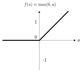
probs = F.softmax(x) All that’s left is to find an image that corresponds to an output with each component being exactly the same in the commented line. One easy first step is to exploit the Rectified Linear Unit (ReLU) activation function, which if you recall looks something like this:
We see it’s a LOT easier to get zeroes in our output than any other number. We set our target for the all zeroes vector as an output for the commented line. However, it turns out that finding an input that corresponds to a given output in a neural network is a really hard problem, and isn’t solvable in general. Thankfully, in our case, the neural network is formed using components that we can throw into a solver (since the network essentially consists of linear components plus the ReLU activation function, which is pretty much linear). Marabou is an SMT-based tooling that allows us to perform queries on the network, for example, we can perform a local robustness query on a network to see if any value in some delta around a given input meets a certain bound, as shown below:
delta = 0.03
# set bounds on input
for h in range(inputVars.shape[0]):
    for w in range(inputVars.shape[1]):
        network.setLowerBound(inputVars[h][w][0], 0.5-delta)
        network.setUpperBound(inputVars[h][w][0], 0.5+delta)

# set bounds on output
network.setLowerBound(outputVars[0], 7.0)

print("Check query with more restrictive output constraint (Should be UNSAT)")
vals, stats = network.solve(options = options)
assert len(vals) == 0
It can also be used to see what input values satisfy the constraint, as returned in vals by the call to network.solve when the solution is satisfiable. However, we can’t just take the model given to us in the challenge (leenet.ph) since PyTorch models aren’t natively supported in Marabou. To avert this problem, we define a DumbNet specifically to export the parameters that we care about (the two linear layers fc1 and fc2) into a format supported by Marabou, which in this case is the .onnx format.
class DumbNet(nn.Module):
    def __init__(self, nFeatures=NFEATURES, nHidden=NHIDDEN, nCl=NCL):
        super().__init__()
        self.fc1 = nn.Linear(nFeatures, nHidden)
        self.fc2 = nn.Linear(nHidden, nCl)

    def forward(self, x):
        # Normal FC network.
        x = F.relu(self.fc1(x))
        x = F.relu(self.fc2(x))

        return x

dumbnet = DumbNet()
for dumbparam, param in zip(dumbnet.parameters(), model.parameters()):
    if dumbparam.requires_grad:
        dumbparam.data = param.data

torch.onnx.export(dumbnet, (x[0]), 'leenet.onnx', verbose=True)
To examine the exact constraints needed for our input, we take a look at the transforms performed on the input image:
transform = transforms.Compose([transforms.Resize(16),
                                transforms.CenterCrop(16),
                                transforms.Grayscale(),
                                transforms.ToTensor()])
The key function to look at is ToTensor, which maps each pixel to a float value from \([0,1]\). Finally, pass the model into Marabou and solve for all outputVars to be zero, taking into account that the image values are constrained to be between 0 and 1. The solve script is provided below:
#!/usr/bin/env python3

from maraboupy import Marabou
import numpy as np

options = Marabou.createOptions(verbosity = 0)

print("Fully Connected Network Example")
filename = "leenet.onnx"
network = Marabou.read_onnx(filename)


inputVars = network.inputVars[0]
outputVars = network.outputVars

# should be from 0 to 1
for i in range(inputVars.shape[0]):
    network.setLowerBound(inputVars[i], 0.0)
    network.setUpperBound(inputVars[i], 1.0)

# all should equal to 0
for outputVar in outputVars:
    network.addEquality([outputVar], [1] , 0.0)

print("Check query with less restrictive output constraint (Should be SAT)")
vals, stats = network.solve(options = options)
assert len(vals) > 0

print(vals)
ans = []
for i in range(inputVars.shape[0]):
    ans.append(vals[i])

print(ans)
Finally, take the ans and transform it into an image with the same transforms as listed above:
im = transforms.ToPILImage()(adv_x.reshape((16,16))).convert("LA")This gives the following image:

Uploading the image, we get the flag (credits to 4yn for the image below)!
Author’s Reflection
The challenge aims to show a relatively obvious issue in applied numerical computing (which studies floating point arithmetic and numerical stability) but perhaps not so often thought about in machine learning. Such edge cases are of great concern especially when we consider how we use the output of the models downstream. In this challenge, I picked an issue in some arbitrary layer in pytorch, but there’s nothing that says that some similar bugs doesn’t exist in other layers. This raises a really subtle issue that makes trustworthy computing in machine learning much harder than classical imperative computing – not only does the implementation need to be correct, the math has to be correct, and there must not be edge cases that trigger undefined behavior brought about by floating point representation at any point in the network, from the implementation of the layers down to the framework itself. There is no work that rigorously studies this as of yet, and my unpublished manuscript aims to elucidate one instantiation of this problem in a mathematically interesting domain. Do look forward to it!
FAQ
How was the model trained?
Answer: It’s trained on random noise, as all good things should be. Sorry, I didn’t bother to find n number of images for each of our celebrities to actually train properly here.
Other Amazing Writeups
Originally, I did a few simple fuzz tests and believed the setting was sufficiently robust against random inputs, but I didn’t get enough time to come up with a way of verifying or preventing other solutions from working before the competition. Though no one managed to craft the exact solution above, I was quite happy to see the participants thinking out of the box and proving me wrong with fuzzing based techniques and even adversarial approaches. I have linked them below for those interested to find out more:
Hack on!